Querying a lot of data real quick
As discussed in AI Agents and Applesauce, I've been passively working on a recipe search engine for the past several years.
The idea is simple: people should be able to discover recipes by any attribute:
- Nutrient information
- Categories and lifestyle
- Preparation
Everyone's lifestyle has different dietary wants or needs. The primary focus of Foodie is to allow people easy access to that information.
While the idea is simple, the implementation less so.
The term "search engine" has an upfront and unsaid requirement, searching needs to be fast. Like blazing fast. To do this, I made a few upfront decisions:
- Cloudflare Workers for the API. Workers run on Cloudflare's edge network — execution is in the data center closest to the user, not in a single region.
- Cold start times are very fast and the free tier is extremely generous.
- PostgreSQL for data storage. It has been discussed to death that all you need is Postgres.
- GIN indexes, array columns, window functions, triggers. It has the primitives to build a search index without bolting on Elasticsearch or a dedicated search service.
- Hosted on Neon with Cloudflare Hyperdrive for connection pooling, which keeps the operational overhead near zero.
- Budget constraints are a feature. This is a passion project — I need to be able to prove out the idea without spending a lot.
I'm going to tip my hand by beginning with where the project is currently at and then backtrack into how we got here.
| Scenario | Response time |
|---|---|
| Search with multiple filters | 21ms |
| Fetch a single recipe with full details | 10ms |
| Fetch 50 recipes with full details | 13ms |
| Search with no filters | 12ms |
Profiled the search API locally at 1M recipes. The above are p50 response times with a cold cache. Every scenario completes in under 25ms. Minimizing latency shaped every design decision on the read path — starting with the schema.
The Denormalized Search Index
The normalized schema has a typical relational structure:
Searching normalized data would involve multi-way JOINs to filter on ingredient sets. Assuming each recipe has 9 ingredients, 1M recipes results in 9M ingredient rows — a cardinality explosion that forces the query planner into aggregations across millions of rows on every request.
Instead, all search queries target a single denormalized Search Index: one row per recipe.
- PostgreSQL
BIGINT[]array columns that hold the set of Food IDs and Tag IDs associated with that recipe. - Scalar columns for numeric filters like macros and cook time.
- GIN indexes on the array columns enable set-containment queries via the
@>operator.
Here's what the Search Index looks like for three recipes:
| Recipe ID | Food IDs | Tag IDs | Protein | Carbs | Fat | Cook Time |
|---|---|---|---|---|---|---|
| 1 | chicken, rice, soy sauce | dinner, keto | 32g | 45g | 12g | 30 min |
| 2 | salmon, lemon, garlic | dinner, high-protein | 41g | 8g | 18g | 25 min |
| 3 | pasta, tomato, basil | vegetarian, quick | 12g | 58g | 9g | 15 min |
Every column the user can search or filter on lives in this one row. When someone searches for "keto recipes with chicken, at least 30g protein", the database checks one table:
FROM   Search Index
WHERE  Food IDs contain [chicken]
  AND  Tag IDs contain [keto]
  AND  Protein >= 30
Row 1 matches. One table, one index scan, done.
The GIN index maintains inverted posting lists. For each Food ID, it stores the set of Recipe IDs that contain it. The @> operator intersects those posting lists, and because the intersection shrinks with each additional term, higher filter selectivity produces faster queries. Three filter terms produce a smaller posting list intersection than one, so adding additional filters actually improves search performance.
Keeping It in Sync
The fundamental risk with any denormalized table is drift.
The Search Index acts as a materialized view of the normalized tables, and every write to those tables needs to be reflected in the index. Pushing that responsibility to the application layer — every code path that writes an ingredient also updates the Search Index — is fragile. The more places that need to "remember" to sync, the more certain it is that one eventually won't.
PostgreSQL triggers eliminate the problem entirely. The application writes to the normalized tables and the triggers fire unconditionally, in the same transaction, regardless of how the row gets written. The Search Index stays consistent without the caller having to know it exists.
The naive approach would be row-level triggers: one fire per inserted row. Import a recipe with 15 ingredients and 5 tags, and that's 20+ trigger executions each re-aggregating the full array from scratch.
Statement-level triggers with transition tables collapse this. Instead of firing per row, the trigger fires once per statement and receives all affected rows. It extracts distinct recipe IDs from the transition table and rebuilds each affected recipe's arrays in a single pass:
The tradeoff is adding write cost for read speed. But statement-level triggers keep that cost proportional to the number of affected recipes, not the number of inserted rows. That's an important distinction. For a read-heavy search workload with batch writes and largely static data, shifting cost from reads to writes is a good exchange.
Measure twice, cut once
Architectural decisions can only be made confidently with accurate data. For this, we need the ability to profile and benchmark different access patterns at different scales.
I tested at three scales: 10K, 100K, and 1M recipes. To allow for quick iteration, all three tiers used synthetic data. The seed script generates recipes with randomized attributes, then assigns each recipe a random subset of the 248 real foods and 49 real tags from the production vocabulary.
Between each scale tier, I restart Postgres entirely. This clears all caches — shared_buffers, the OS page cache, and query plan caches. Every tier starts cold.
Within a tier, each scenario runs 3 warmup iterations (discarded) followed by 50 measured iterations. The warmup lets the buffer pool load a representative working set for that data size — not fully warm, but past the worst cold-start penalties. This means the p50 numbers reflect realistic warmed-up performance, while the p99 numbers still capture cold-page penalties from early iterations.
The local environment uses Docker Postgres (2GB shared_buffers) and miniflare for the Worker runtime. Critically, miniflare creates a new Postgres connection for every request — no connection pooling at all. That means every measurement includes TCP connection setup, which inflates absolute numbers but makes the benchmark conservative. Production uses Hyperdrive connection pooling, so real latencies will be lower.
The profiler covers 12 scenarios across the API's surface area — from broad unfiltered searches down to single recipe lookups. Each response body includes a query_time_ms field measured server-side with performance.now(), giving me a latency decomposition (database time vs Worker overhead) for every request.
Iterating on the Read Path
The Search Index provides recipe IDs. But a consumer needs full records — name, ingredients, tags, nutrition. That's the hydration step: take a page of IDs and fan out to the normalized tables. Hydration is where most of the latency lives, and it's where the profiling data drove two rounds of optimization.
Per-recipe hydration
The first implementation was the obvious one: for each recipe ID returned by the search, query its ingredients, tags, and nutrition individually. Simple, correct, and painfully slow. At 1M recipes, an unfiltered search took ~190ms of database time. A 50-recipe detail fetch hit ~280ms.
The profiling data made the bottleneck obvious — the round-trip overhead of issuing queries per recipe per table added compounding latency.
Batched hydration
Instead of N queries per table, batch all recipe IDs into a single IN(...) clause per table. Four parallel queries replace dozens of sequential ones:
recipes, ingredients, tags, nutrients = parallel(
    SELECT * FROM Recipe       WHERE id IN recipeIds,
    SELECT * FROM Ingredient   WHERE recipe_id IN recipeIds,
    SELECT * FROM Tag          WHERE recipe_id IN recipeIds,
    SELECT * FROM Nutrition    WHERE recipe_id IN recipeIds,
)
Re-profiling at 1M showed the improvement immediately. Unfiltered search dropped from ~190ms to 53ms. The 50-recipe detail fetch went from ~280ms to 17ms. Batching eliminated the per-recipe round-trip overhead, and the result set is bounded by batch size, not table cardinality — detail fetches are effectively constant-time in data size.
The profiling data also revealed a useful property of the GIN index: higher selectivity produces faster queries. Searching with all filters at 1M (27ms) outperformed a single food filter (45ms) because additional filter terms shrink the posting list intersection. Adding filter complexity improves query performance, which is the opposite of what happens with multi-table JOINs.
But the data raised another question. If recipe data is largely static, why rebuild the same hydrated response from 4 tables on every request?
Materialized hydration
The solution: a pre-built cache table with one row per recipe and a single JSONB column containing the fully hydrated record. Hydration goes from 4 parallel queries to 1:
cached = SELECT hydrated_json FROM RecipeCache WHERE id IN recipeIdsThe same statement-level trigger pattern that keeps the Search Index in sync also maintains the cache. A batch write to ingredients, tags, or nutrition rebuilds the cached JSONB for all affected recipes in a single pass.
The full picture
Three rounds of profiling, three hydration strategies. Each optimization was driven by the previous round's data:
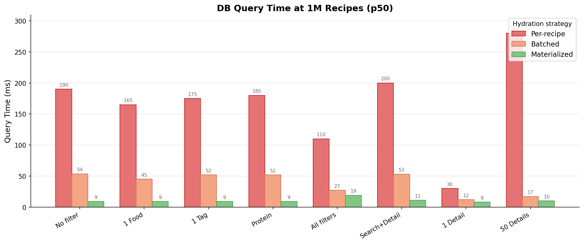
End-to-end reductions range from 83% to 96% across scenarios. The biggest wins came from eliminating round-trip overhead (per-recipe to batched). Materialization then collapsed the remaining fan-out, with the largest gains on broad, low-selectivity queries. Tail latency improved just as dramatically — the worst p99 dropped from 171ms to 39ms.
The tradeoffs
The cache isn't free. Every recipe's data now lives in three places: normalized tables, Search Index, and cache. That's storage duplication and write amplification — each batch write fires statement-level triggers for both the Search Index and the cache. And the cache's JSONB structure mirrors the API response contract, so any schema evolution means rebuilding every cached row.
These costs land well here because of three properties:
- Largely static data. Recipes don't change after import. Cache invalidation — the classic hard problem — barely applies when the underlying data rarely mutates. A social feed or live inventory with frequent writes would pay the trigger cost on every mutation.
- Read-heavy workload. The cache pays its write cost once during import and recoups it on every search result page, detail view, and comparison card. A write-heavy workload with few reads would never recoup.
- Batch write pipeline. Recipes are imported in bulk. Statement-level triggers already keep the per-statement cost low, but for very large imports the triggers can be disabled entirely and the index and cache rebuilt in one pass afterwards.
Building the Profiling Harness with Claude Code
The entire profiling suite — seed generation, benchmark runner, report generator, backup/restore tooling — is about 1,000 lines of Python across four scripts. I built all of it in under two hours using Claude Code. The scope wasn't trivial: the seed script generates realistic data across six related tables with triggers disabled for bulk performance, the benchmark runner hits 12 API scenarios capturing both HTTP and server-side timing, and the report generator computes percentile statistics across scale tiers.
The back-and-forth was fast because Claude Code could read the schema and API routes directly — it generated code that matched actual table structures and endpoint contracts without me specifying every column name. I described what I wanted, reviewed the output, and iterated on edge cases like flushing the buffer pool between tiers and extracting query_time_ms from response bodies.
The profiling harness is what made materialized hydration possible — without concrete data showing that DB time dominated the critical path and hydration was the bottleneck, I'd have been going on instinct. Being able to offload profiling while working in parallel was huge.
Takeaways
Denormalize the search path. A single table with array columns and GIN indexes is dramatically simpler to query and optimize than multi-table JOINs. Pay the write-time cost with triggers, recoup it on every read. For search workloads backed by batch write pipelines, this tradeoff isn't even close.
Understand your index's access pattern. GIN posting list intersection means more filter terms = faster queries. That's a property of the index structure, not an accident. Choosing the right index type requires understanding the query patterns it will serve, not just which columns to index.
Trade write cost for read speed — when the data lets you. Two rounds of hydration optimization reduced query times by 83-96%. But the cache introduces storage duplication, write amplification, and schema coupling. That tradeoff lands well for static data with batch writes and high read volume. It would be the wrong choice for frequently-mutating data or unbounded payloads.
Decompose latency along the critical path. When you can see that the Worker adds less than 5ms of overhead and the rest is database time, you know exactly where to focus. Without that observability, you'd waste time optimizing the wrong layer.